Webarc:Packaging: Difference between revisions
From Adapt
No edit summary |
No edit summary |
||
| (10 intermediate revisions by the same user not shown) | |||
| Line 17: | Line 17: | ||
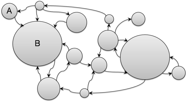
Although simple and straightforward, one problem with this simple packaging approach appears at access time. That is, tightly related pages can end up in different containers, and more number of containers will be necessary in a random browsing session. | Although simple and straightforward, one problem with this simple packaging approach appears at access time. That is, tightly related pages can end up in different containers, and more number of containers will be necessary in a random browsing session. | ||
[[Image:conv_container_packaging.png| | [[Image:conv_container_packaging.png|480px]] | ||
== Our Goal == | == Our Goal == | ||
We aim to develop a methodology to minimize the probability that a user jumps often between containers when accessing the web archive. | We aim to develop a methodology to minimize the probability that a user jumps often between containers when accessing the web archive. | ||
[[Image:ideal_container_packaging.png| | [[Image:ideal_container_packaging.png|480px]] | ||
== Our Approach == | == Our Approach == | ||
| Line 28: | Line 28: | ||
Based on PageRank, we compute EdgeRank for each edge that represents the global probability of the edge to be taken. | Based on PageRank, we compute EdgeRank for each edge that represents the global probability of the edge to be taken. | ||
<math> EdgeRank(u) = \frac{ \displaystyle \frac{1-d}{N} + d \sum_{v \in I_u} p_{vu} PR(v)}{outdegree(v)}</math>, where <math>N</math> is the number of pages, <math>d</math> is a damping factor (=0.15), <math>I_u</math> is a set of pages that have hyperlinks to Page <math>u</math>, <math>p_{vu}</math> is the probability of the hyperlink from Page <math>v</math> to Page <math>u</math> to be taken, and <math>PR(v)</math> is the PageRank of Page <math>v</math> | <center><math> EdgeRank(u) = \frac{ \displaystyle \frac{1-d}{N} + d \sum_{v \in I_u} p_{vu} PR(v)}{outdegree(v)}</math></center> | ||
, where <math>N</math> is the number of pages, <math>d</math> is a damping factor (=0.15), <math>I_u</math> is a set of pages that have hyperlinks to Page <math>u</math>, <math>p_{vu}</math> is the probability of the hyperlink from Page <math>v</math> to Page <math>u</math> to be taken, and <math>PR(v)</math> is the PageRank of Page <math>v</math> | |||
=== Graph Partitioning Technique === | === Graph Partitioning Technique === | ||
Given a directed web graph | Given a directed web graph with weighted nodes and edges, we determine a partition, such that | ||
# Edge-Cut is minimized. | # Edge-Cut is minimized. | ||
# The sum of node weights in each part is upper bounded by some K. | # The sum of node weights in each part is upper bounded by some K. | ||
| Line 41: | Line 43: | ||
# Compute minimum edge-cut bisection. | # Compute minimum edge-cut bisection. | ||
# Refine and uncoarsen the partitioned graph. | # Refine and uncoarsen the partitioned graph. | ||
== Experiments == | |||
* Datasets | |||
** UMIACS: Web Graph built from our crawls of http://umiacs.umd.edu in 2007 | |||
** Stanford: Web Graph built from a crawl of http://stanford.edu in 2002 by the Stanford WebBase project | |||
{| class="wikitable" border="1" align="center" | |||
|- | |||
! Datasets | |||
! # Vertices | |||
! # Edges | |||
! Total Vertex Weight | |||
|- | |||
! UMIACS Web Graph | |||
| align="right" | 4579 | |||
| align="right" | 9732 | |||
| align="right" | 2.49GB | |||
|- | |||
! Stanford Web Graph | |||
| align="right" | 281903 | |||
| align="right" | 2312497 | |||
| align="right" | 215.82GB | |||
|} | |||
* Three Packaging Methods | |||
** CONV: Pages are allocated to containers as they are fetched during the crawling process (BFS). Once a container is full, we use a new container. | |||
** GP: The graph partitioning technique is applied so as to minimize the number of edges connecting any two partitions. All the pages belonging to a partition are allocated to a single container. | |||
** ER+GP: EdgeRank is used to assign weights to edges, and the graph is partitioned using a minimum-weight partitioning algorithm. | |||
* Edge-Cut Result | |||
<center><math> EdgeCut_{scaled} = \frac{EdgeCut*100}{Number of Edges}</math></center> | |||
{| class="wikitable" border="1" align="center" | |||
|- | |||
! align="center" rowspan="2" | EdgeCut | |||
! align="center" colspan="2" | Unweighted Edges | |||
! align="center" colspan="2" | Weighted Edges | |||
|- | |||
! align="center" | CONV | |||
! align="center" | GP | |||
! align="center" | ER+CONV | |||
! align="center" | ER+GP | |||
|- | |||
! align="center" | UMIACS Web Graph | |||
| align="center" | 73.87 | |||
| align="center" | 12.38 | |||
| align="center" | 62.36 | |||
| align="center" | 36.03 | |||
|- | |||
! align="center" | Stanford Web Graph | |||
| align="center" | 80.50 | |||
| align="center" | 47.33 | |||
| align="center" | 63.56 | |||
| align="center" | 32.20 | |||
|} | |||
=== Simulation === | |||
* Simulation Parameters | |||
{| class="wikitable" border="1" align="center" | |||
|- | |||
! align="center" | Parameter | |||
! align="center" | Value | |||
|- | |||
! align="center" | Number of Random Walks | |||
| align="center" | 1000 | |||
|- | |||
! align="center" | Number of Hops in Each Walk | |||
| align="center" | 10 | |||
|- | |||
! align="center" | Probability of Going Back | |||
| align="center" | 30% | |||
|- | |||
! align="center" | Out-degree of Starting Vertex | |||
| align="center" | >5 | |||
|- | |||
! align="center" | Policy at Dangling Vertex | |||
| align="center" | Go Back | |||
|} | |||
* Simulation Results | |||
We run 1000 random walks. In each random walk, we let a user hop 10 times randomly in the web graph. The following histograms show the number of random walks (out of 1000) in the y-axis for the number of inter-container hops and distinct containers, respectively. The first two histograms are for the UMIACS web graph, and the next two histograms are for the Stanford web graph. In any case, it is clear that GP and ER+GP techniques required fewer number of inter-container hops as well as distinct containers. For example, the first histogram shows that more than 600 random walks (out of 1000) needed only a single container when ER+GP was applied in the UMIACS web graph. | |||
[[Image:umiacs_ih.png|640px]] | |||
[[Image:umiacs_dc.png|640px]] | |||
[[Image:stanford_ih.png|640px]] | |||
[[Image:stanford_dc.png|640px]] | |||
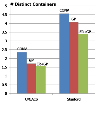
The following two graphs show the average number of inter-container hops and distinct containers, respectively. | |||
[[Image:avg_ih.png|320px]][[Image:avg_dc.png|320px]] | |||
== Publication == | |||
Song, S. and JaJa, J. Fast Browsing of Archived Web Contents. in 8th International Web Archiving Workshop. 2008. Aarhus, Denmark. [[media:iwaw08_Song_JaJa_Final.pdf|pdf]] | |||
Latest revision as of 22:43, 24 September 2008
Background
Web Graph
Web can be considered as a weighted, directed graph where web pages are vertices and hyperlinks are edges in the graph. The size of a page is the weight of the corresponding vertex.
Web Containers
There are many different ways to archive the web. One of the most popular methods is through use of containers. In this container method, a multitude of web pages are aggregated into a container. An emerging standard for such containers is the WARC format, which evolved from the ARC container format developed by the Internet Archive, currently the world’s largest internet archive.
Motivation
Conventional Container Packaging
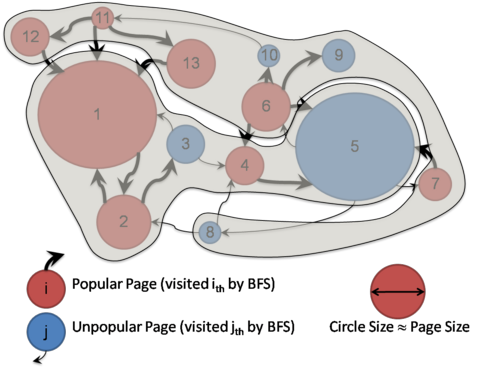
The conventional way to construct containers is rather naive. Most web crawls are based on Breadth First Search or Depth First Search, and throughout the crawl session, first seen pages are put into a container until the container gets full. When the container gets full, a new container is created for the pages to be seen next. The process repeats itself until the crawl session ends.
Problem with the Conventional Container Packaging
Although simple and straightforward, one problem with this simple packaging approach appears at access time. That is, tightly related pages can end up in different containers, and more number of containers will be necessary in a random browsing session.
Our Goal
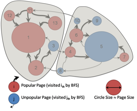
We aim to develop a methodology to minimize the probability that a user jumps often between containers when accessing the web archive.
Our Approach
Graph Analysis Technique
Based on PageRank, we compute EdgeRank for each edge that represents the global probability of the edge to be taken.
, where <math>N</math> is the number of pages, <math>d</math> is a damping factor (=0.15), <math>I_u</math> is a set of pages that have hyperlinks to Page <math>u</math>, <math>p_{vu}</math> is the probability of the hyperlink from Page <math>v</math> to Page <math>u</math> to be taken, and <math>PR(v)</math> is the PageRank of Page <math>v</math>
Graph Partitioning Technique
Given a directed web graph with weighted nodes and edges, we determine a partition, such that
- Edge-Cut is minimized.
- The sum of node weights in each part is upper bounded by some K.
Since this is an NP-complete problem, we apply a heuristic algorithm. In our experiments, we choose an algorithm introduced by Karypis and Kumar in 1998 known as Fast Multilevel Graph Partitioning Algorithm. Below is the overview of the algorithm.
- Compute a maximal matching using a randomized algorithm.
- Coarsen the graph by collapsing the matched vertices together.
- Repeat Step 1~2 until a desired size of the coarsened graph is achieved.
- Compute minimum edge-cut bisection.
- Refine and uncoarsen the partitioned graph.
Experiments
- Datasets
- UMIACS: Web Graph built from our crawls of http://umiacs.umd.edu in 2007
- Stanford: Web Graph built from a crawl of http://stanford.edu in 2002 by the Stanford WebBase project
| Datasets | # Vertices | # Edges | Total Vertex Weight |
|---|---|---|---|
| UMIACS Web Graph | 4579 | 9732 | 2.49GB |
| Stanford Web Graph | 281903 | 2312497 | 215.82GB |
- Three Packaging Methods
- CONV: Pages are allocated to containers as they are fetched during the crawling process (BFS). Once a container is full, we use a new container.
- GP: The graph partitioning technique is applied so as to minimize the number of edges connecting any two partitions. All the pages belonging to a partition are allocated to a single container.
- ER+GP: EdgeRank is used to assign weights to edges, and the graph is partitioned using a minimum-weight partitioning algorithm.
- Edge-Cut Result
| EdgeCut | Unweighted Edges | Weighted Edges | ||
|---|---|---|---|---|
| CONV | GP | ER+CONV | ER+GP | |
| UMIACS Web Graph | 73.87 | 12.38 | 62.36 | 36.03 |
| Stanford Web Graph | 80.50 | 47.33 | 63.56 | 32.20 |
Simulation
- Simulation Parameters
| Parameter | Value |
|---|---|
| Number of Random Walks | 1000 |
| Number of Hops in Each Walk | 10 |
| Probability of Going Back | 30% |
| Out-degree of Starting Vertex | >5 |
| Policy at Dangling Vertex | Go Back |
- Simulation Results
We run 1000 random walks. In each random walk, we let a user hop 10 times randomly in the web graph. The following histograms show the number of random walks (out of 1000) in the y-axis for the number of inter-container hops and distinct containers, respectively. The first two histograms are for the UMIACS web graph, and the next two histograms are for the Stanford web graph. In any case, it is clear that GP and ER+GP techniques required fewer number of inter-container hops as well as distinct containers. For example, the first histogram shows that more than 600 random walks (out of 1000) needed only a single container when ER+GP was applied in the UMIACS web graph.
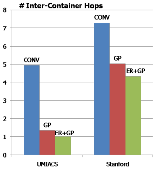
The following two graphs show the average number of inter-container hops and distinct containers, respectively.
Publication
Song, S. and JaJa, J. Fast Browsing of Archived Web Contents. in 8th International Web Archiving Workshop. 2008. Aarhus, Denmark. pdf
